บทนำสู่ Qiskit

ใน notebook นี้เราจะสำรวจวิธีการเขียนโปรแกรม quantum gates และ quantum circuits ด้วย Qiskit รวมถึงวิธีรันบน simulator และคอมพิวเตอร์ควอนตัมจริงโดยใช้ Qiskit patterns ต่อจากนั้นเราจะแนะนำวิธีการต่าง ๆ ในการเข้ารหัสข้อมูล และปิดท้ายด้วยตัวอย่างโบนัสของ Quantum Teleportation

ก่อนเริ่มต้น

ทำตามขั้นตอน ติดตั้งและตั้งค่า ถ้ายังไม่ได้ทำ รวมถึงขั้นตอน ตั้งค่าเพื่อใช้งาน IBM Quantum™ Platform

แนะนำให้ใช้สภาพแวดล้อมการพัฒนา Jupyter เพื่อโต้ตอบกับคอมพิวเตอร์ควอนตัม อย่าลืมติดตั้ง visualization support เพิ่มเติมที่แนะนำ ('qiskit[visualization]') นอกจากนี้ยังต้องใช้ package matplotlib สำหรับตัวอย่างในส่วนที่สองด้วย

หากอยากเรียนรู้เรื่อง quantum computing โดยทั่วไป แวะดูที่ Basics of quantum information course บน IBM Quantum Learning

Imports

# Added by doQumentation — required packages for this notebook
!pip install -q matplotlib numpy qiskit qiskit-aer qiskit-ibm-runtime

# Import necessary modules for this notebook
import time
import qiskit

from qiskit import QuantumCircuit
from qiskit.quantum_info import Statevector
from qiskit.visualization import plot_bloch_multivector, plot_state_qsphere
from qiskit_aer import AerSimulator
from qiskit.quantum_info import SparsePauliOp
from qiskit.transpiler.preset_passmanagers import generate_preset_pass_manager
from qiskit_ibm_runtime import EstimatorV2 as Estimator
from qiskit_ibm_runtime import SamplerV2 as Sampler
from qiskit_ibm_runtime import QiskitRuntimeService
from qiskit.visualization import plot_histogram
print(qiskit.__version__)

2.3.1

ในการรัน quantum circuits บน hardware จำเป็นต้องตั้งค่าบัญชีก่อน ทำได้ดังนี้:

1. ไปที่ IBM Quantum® Platform เวอร์ชันใหม่
2. ไปที่มุมขวาบน (ดูรูปด้านบน) สร้าง API token แล้วคัดลอกไปเก็บไว้ในที่ปลอดภัย
3. ในเซลล์ถัดไป แทนที่ deleteThisAndPasteYourAPIKeyHere ด้วย API key ของตัวเอง
4. ไปที่มุมซ้ายล่าง (ดูรูปด้านบน) แล้ว สร้าง instance โดยเลือก open plan
5. หลังสร้าง instance แล้ว คัดลอก CRN code ที่เชื่อมกับ instance นั้น อาจต้องรีเฟรชเพื่อให้เห็น instance
6. ในเซลล์ด้านล่าง แทนที่ deleteThisAndPasteYourCRNHere ด้วย CRN code

ดู คู่มือนี้ สำหรับรายละเอียดเพิ่มเติมเกี่ยวกับการตั้งค่าบัญชี IBM Cloud®

⚠️ หมายเหตุ: ดูแล API key เหมือนกับรหัสผ่านที่ต้องรักษาความปลอดภัย ดู คู่มือ Cloud setup สำหรับข้อมูลเพิ่มเติมเกี่ยวกับการใช้ API key ในสภาพแวดล้อมที่ปลอดภัยและไม่ปลอดภัย

#your_api_key = "deleteThisAndPasteYourAPIKeyHere"
#your_crn = "deleteThisAndPasteYourCRNHere"

QiskitRuntimeService.save_account(
    channel="ibm_quantum_platform",
    token=your_api_key,
    instance=your_crn,
    overwrite=True
)

1. Quantum Gates และ Quantum Circuits

Quantum circuits เป็นโมเดลสำหรับการคำนวณควอนตัม ซึ่งการคำนวณคือลำดับของ quantum gates มาดู quantum gates ที่นิยมใช้กันบ้าง

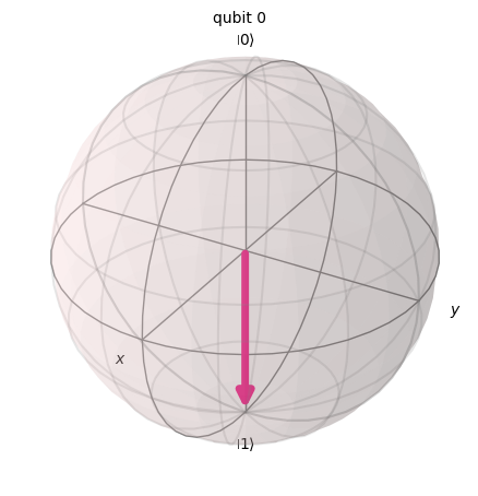
X Gate

X gate เทียบเท่ากับการหมุนรอบแกน X ของ Bloch sphere เป็นมุม $\pi$ เรเดียน มันแปลง $|0\rangle$ เป็น $|1\rangle$ และ $|1\rangle$ เป็น $|0\rangle$ ถือเป็น quantum equivalent ของ NOT gate ในคอมพิวเตอร์แบบคลาสสิก บางครั้งเรียกว่า bit-flip

$X = \begin{pmatrix} 0 & 1 \\ 1 & 0 \\ \end{pmatrix}$

# Let's apply an X-gate on a |0> qubit
qc = QuantumCircuit(1)
qc.x(0)
qc.draw(output='mpl')

# Let's see Bloch sphere visualization
sv = Statevector(qc)
plot_bloch_multivector(sv)

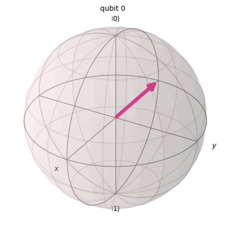
H Gate

Hadamard gate คือการหมุนรอบแกนที่อยู่ระหว่างแกน $X$ และแกน $Z$ เป็นมุม $\pi$ มันแปลง basis state $|0\rangle$ เป็น $\frac{|0\rangle + |1\rangle}{\sqrt{2}}$ ซึ่งหมายความว่าการวัดจะมีโอกาสเป็น 1 หรือ 0 เท่ากัน สร้าง 'superposition' ของสถานะ สถานะนี้เขียนได้อีกแบบว่า $|+\rangle$

$H = \frac{1}{\sqrt{2}}\begin{pmatrix} 1 & 1 \\ 1 & -1 \\ \end{pmatrix}$

# Let's apply an H-gate on a |0> qubit
qc = QuantumCircuit(1)
qc.x(0)
qc.h(0)
qc.draw(output='mpl')

# Let's see Bloch sphere visualization
sv = Statevector(qc)
plot_bloch_multivector(sv)

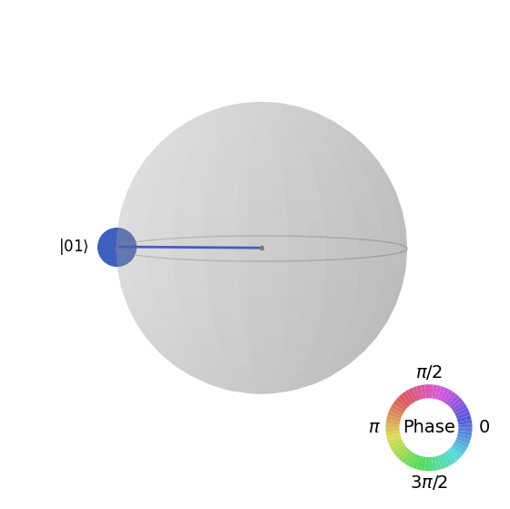
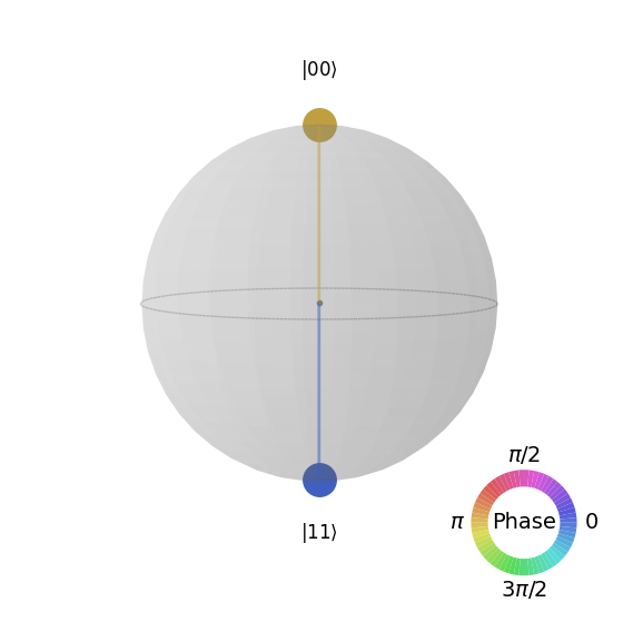
CX Gate (CNOT Gate)

CNOT (หรือ CX) gate ทำงานกับ qubit สองตัว โดยจะทำการ NOT (เทียบเท่ากับการใช้ X gate) กับ qubit ตัวที่สองก็ต่อเมื่อ qubit ตัวแรกเป็น $|1\rangle$ ถ้าไม่ใช่ก็จะปล่อยไว้เหมือนเดิม หมายเหตุ: Qiskit นับบิตในสตริงจากขวาไปซ้าย

$CX = \begin{pmatrix} 1 & 0 & 0 & 0\\ 0 & 1 & 0 & 0\\ 0 & 0 & 0 & 1\\ 0 & 0 & 1 & 0\\ \end{pmatrix}$

# Let's apply a CX-gate on |11>
qc = QuantumCircuit(2)
qc.x(0)
qc.x(1)
qc.cx(0,1)
qc.draw(output='mpl')

sv=Statevector(qc)
plot_state_qsphere(sv)

สร้าง Bell state แรก

$|\phi^+ \rangle = \frac{1}{\sqrt 2}(|00 \rangle + |11 \rangle)$

# Create a Bell state circuit

qc = QuantumCircuit(2)
qc.h(0)
qc.cx(0,1)

# Draw the circuit
qc.draw("mpl")

# Plot the state using q-sphere visualization
sv = Statevector(qc)
plot_state_qsphere(sv)
# q-sphere is useful for visualizing states when Bloch sphere fails to

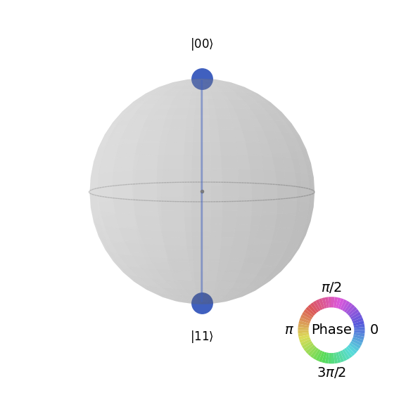
สร้าง Bell state ที่สอง

$|\phi^- \rangle = \frac{1}{\sqrt 2}(|00 \rangle - |11 \rangle)$

# Create a circuit with the second Bell state

qc = QuantumCircuit(2)
qc.x(0)
qc.h(0)
qc.cx(0,1)

qc.draw("mpl")

คำอธิบายคือ:

$$H|1\rangle=\frac{1}{\sqrt{2} }(|0\rangle-|1\rangle) = |-\rangle$$

# Get the statevector of the circuit
sv = Statevector(qc)

# Plot the state using qsphere visualization
plot_state_qsphere(sv)

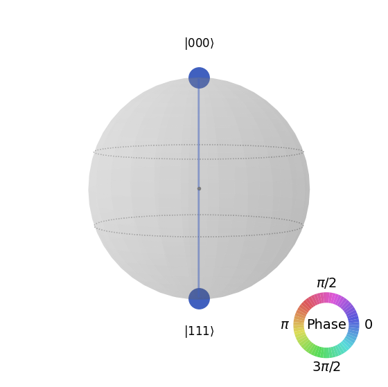
สร้าง 3-qubit GHZ state

$|GHZ \rangle = \frac{1}{\sqrt 2}(|000 \rangle + |111 \rangle)$

# Create a circuit with 3-qubit GHZ state

qc= QuantumCircuit(3)
qc.h(0)
qc.cx(0,1)
qc.cx(0,2)

qc.draw("mpl")

# Get the statevector of the circuit
sv = Statevector(qc)

# Plot the state using qsphere visualization
plot_state_qsphere(sv)

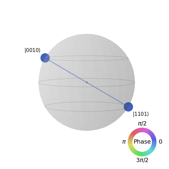
สร้าง Qiskit logo state

$|Qiskit \rangle = \frac{1}{\sqrt 2}(|0010 \rangle + |1101 \rangle)$

# Create a circuit with the Qiskit logo state

qc = QuantumCircuit(4)
qc.h(0)
qc.cx(0,1)
qc.cx(0,2)
qc.cx(0,3)
qc.x(1)

# Draw the circuit
qc.draw("mpl")

# Get the statevector of the circuit
sv = Statevector(qc)

# Plot the state using qsphere visualization
plot_state_qsphere(sv)

2. สร้างและรันโปรแกรมควอนตัมอย่างง่าย

สี่ขั้นตอนในการเขียนโปรแกรมควอนตัมโดยใช้ Qiskit patterns ได้แก่:

1. แปลงปัญหาให้อยู่ในรูปแบบ quantum-native

2. ปรับปรุง Circuit และ operator ให้เหมาะสม

3. รันด้วยฟังก์ชัน quantum primitive

4. วิเคราะห์ผลลัพธ์

2.1 Map the problem to a quantum-native format

ในโปรแกรมควอนตัม quantum circuits คือรูปแบบดั้งเดิมที่ใช้แทนคำสั่งควอนตัม และ operators คือออบเซิร์ฟเวเบิลที่ต้องการวัด เวลาสร้าง Circuit มักจะสร้าง object QuantumCircuit ใหม่ แล้วค่อยเพิ่มคำสั่งเข้าไปทีละขั้น

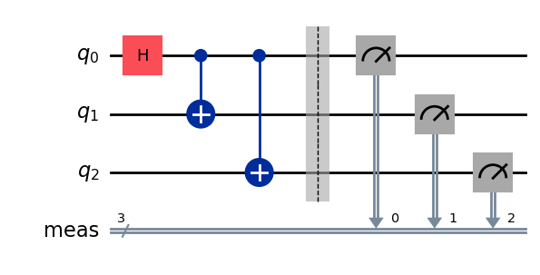
โค้ดด้านล่างสร้าง Circuit ที่ผลิต GHZ state ซึ่งเป็นสถานะที่ Qubit สาม Qubit พันกันอย่างสมบูรณ์

Qiskit SDK ใช้ระบบเลข LSb 0 ที่ตัวเลขหลักที่ $n$ มีค่าเท่ากับ $1 \ll n$ หรือ $2^n$ ดูรายละเอียดเพิ่มเติมได้ที่หัวข้อ Bit-ordering in the Qiskit SDK

# Create a GHZ state circuit

qc = QuantumCircuit(3)
qc.h(0)
qc.cx(0,1)
qc.cx(0,2)
# Draw the circuit
qc.draw("mpl")

ดูการดำเนินการทั้งหมดที่ใช้ได้ใน QuantumCircuit จากเอกสาร

เวลาสร้าง quantum circuits ต้องคิดด้วยว่าอยากได้ข้อมูลแบบไหนหลังรัน Qiskit มีสองวิธีในการคืนค่า: ได้การกระจายความน่าจะเป็นของ Qubit ชุดที่เลือกวัด หรือได้ค่าคาดหวังของออบเซิร์ฟเวเบิล เตรียม workload ให้วัด Circuit ในหนึ่งในสองแบบนี้ด้วย Qiskit primitives (อธิบายละเอียดในขั้นที่ 3)

ตัวอย่างนี้วัดค่าคาดหวังโดยใช้ submodule qiskit.quantum_info ซึ่งระบุด้วย operators (ออบเจกต์ทางคณิตศาสตร์ที่แทนการกระทำหรือกระบวนการที่เปลี่ยนสถานะควอนตัม) โค้ดด้านล่างสร้าง Pauli operators สามตัว-Qubit จำนวนหกตัวได้แก่ ZZZ, ZZX, ZII, XXI, ZZI และ III

# Set up six different observables.

observables_labels = ["ZZZ", "ZZX", "ZII", "XXI", "ZZI", "III"]

observables = [SparsePauliOp(label) for label in observables_labels]
print(observables)

[SparsePauliOp(['ZZZ'],
              coeffs=[1.+0.j]), SparsePauliOp(['ZZX'],
              coeffs=[1.+0.j]), SparsePauliOp(['ZII'],
              coeffs=[1.+0.j]), SparsePauliOp(['XXI'],
              coeffs=[1.+0.j]), SparsePauliOp(['ZZI'],
              coeffs=[1.+0.j]), SparsePauliOp(['III'],
              coeffs=[1.+0.j])]

ZZI operator นั้นเป็นชื่อย่อของ tensor product $Z\otimes Z\otimes I$ ซึ่งหมายถึงการวัด Z บน Qubit 2 และ Z บน Qubit 1 พร้อมกัน และได้ข้อมูลเกี่ยวกับความสัมพันธ์ระหว่าง Qubit 2 กับ Qubit 1 ค่าคาดหวังแบบนี้มักเขียนว่า $\langle Z_2 Z_1 \rangle$

ถ้าสถานะที่สังเกตคือ GHZ state สามตัว-Qubit การวัด $\langle Z_2 Z_1 \rangle$ ควรได้ค่าเท่ากับ 1

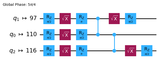
2.2 Optimize the circuits and operators

เวลารัน circuits บนอุปกรณ์ สิ่งสำคัญคือต้องปรับชุดคำสั่งใน Circuit ให้เหมาะสมและลด depth โดยรวม (คร่าว ๆ คือจำนวนคำสั่ง) ของ Circuit เพื่อให้ได้ผลลัพธ์ที่ดีที่สุดโดยลดผลกระทบจาก error และ noise นอกจากนี้คำสั่งใน Circuit ยังต้องเป็นไปตาม Instruction Set Architecture (ISA) ของ Backend และต้องคำนึงถึง basis gates และการเชื่อมต่อของ Qubit ในอุปกรณ์นั้นด้วย

โค้ดด้านล่างสร้าง instance ของอุปกรณ์จริงเพื่อส่ง job และแปลง Circuit กับ observables ให้ตรงกับ ISA ของ Backend นั้น ถ้ายังไม่เคยบันทึก credentials ไว้ ดูวิธียืนยันตัวตนด้วย API token ได้ที่นี่

# Choose a real backend
service = QiskitRuntimeService(channel='ibm_quantum_platform',)
backend = service.least_busy(min_num_qubits=156)
# print backend details
print(
    f"Name: {backend.name}\n"
    f"Version: {backend.backend_version}\n"
    f"No. of qubits: {backend.num_qubits}\n"
    f"Processor type: {backend.processor_type}\n"
)

Name: ibm_marrakesh
Version: 1.0.21
No. of qubits: 156
Processor type: {'family': 'Heron', 'revision': '2'}

# option to use the AerSimulator instead of a real quantum device
seed_sim=42
backend=AerSimulator.from_backend(backend,seed_simulator=seed_sim)

Transpile the circuit into ISA circuit

# Convert to an ISA circuit and layout-mapped observables.

pm = generate_preset_pass_manager(backend=backend, optimization_level=2)
isa_circuit = pm.run(qc) 

isa_circuit.draw("mpl", idle_wires=False)

mapped_observables = [
    observable.apply_layout(isa_circuit.layout) for observable in observables
]
print(mapped_observables)

[SparsePauliOp(['IIIIIIIIIIIIIIIIZIIIIIZIIIIIIIIIIIIZIIIIIIIIIIIIIIIIIIIIIIIIIIIIIIIIIIIIIIIIIIIIIIIIIIIIIIIIIIIIIIIIIIIIIIIIIIIIIIIIIIIIIIIIIIIIIIIII'],
              coeffs=[1.+0.j]), SparsePauliOp(['IIIIIIIIIIIIIIIIZIIIIIXIIIIIIIIIIIIZIIIIIIIIIIIIIIIIIIIIIIIIIIIIIIIIIIIIIIIIIIIIIIIIIIIIIIIIIIIIIIIIIIIIIIIIIIIIIIIIIIIIIIIIIIIIIIIII'],
              coeffs=[1.+0.j]), SparsePauliOp(['IIIIIIIIIIIIIIIIZIIIIIIIIIIIIIIIIIIIIIIIIIIIIIIIIIIIIIIIIIIIIIIIIIIIIIIIIIIIIIIIIIIIIIIIIIIIIIIIIIIIIIIIIIIIIIIIIIIIIIIIIIIIIIIIIIIII'],
              coeffs=[1.+0.j]), SparsePauliOp(['IIIIIIIIIIIIIIIIXIIIIIIIIIIIIIIIIIIXIIIIIIIIIIIIIIIIIIIIIIIIIIIIIIIIIIIIIIIIIIIIIIIIIIIIIIIIIIIIIIIIIIIIIIIIIIIIIIIIIIIIIIIIIIIIIIIII'],
              coeffs=[1.+0.j]), SparsePauliOp(['IIIIIIIIIIIIIIIIZIIIIIIIIIIIIIIIIIIZIIIIIIIIIIIIIIIIIIIIIIIIIIIIIIIIIIIIIIIIIIIIIIIIIIIIIIIIIIIIIIIIIIIIIIIIIIIIIIIIIIIIIIIIIIIIIIIII'],
              coeffs=[1.+0.j]), SparsePauliOp(['IIIIIIIIIIIIIIIIIIIIIIIIIIIIIIIIIIIIIIIIIIIIIIIIIIIIIIIIIIIIIIIIIIIIIIIIIIIIIIIIIIIIIIIIIIIIIIIIIIIIIIIIIIIIIIIIIIIIIIIIIIIIIIIIIIIII'],
              coeffs=[1.+0.j])]

2.3 Execute using the quantum primitives

คอมพิวเตอร์ควอนตัมสามารถให้ผลลัพธ์แบบสุ่มได้ ดังนั้นปกติเราจะเก็บตัวอย่างผลลัพธ์โดยรัน Circuit หลายครั้ง ค่าคาดหวังของ observable สามารถประมาณได้โดยใช้คลาส Estimator Estimator เป็นหนึ่งในสอง primitives อีกอันคือ Sampler ซึ่งใช้ดึงข้อมูลจากคอมพิวเตอร์ควอนตัมได้ object เหล่านี้มี method run() ที่รัน circuits, observables และพารามิเตอร์ที่เลือก (ถ้ามี) โดยใช้ primitive unified bloc (PUB) เวลารันโค้ดนี้บน quantum hardware จริง ควรพิจารณาใช้ เทคนิค error mitigation และ suppression เพื่อลด noise ที่มีอยู่ในตัวของคอมพิวเตอร์ควอนตัม

# Construct the Estimator instance.
estimator = Estimator(mode=backend)
estimator.options.resilience_level = 1
estimator.options.default_shots = 5000

ส่ง job โดยใช้ Estimator primitive

# One pub, with one circuit to run against six different observables.
job = estimator.run([(isa_circuit, mapped_observables)]) 

# Use the job ID to retrieve your job data later
print(f">>> Job ID: {job.job_id()}")

>>> Job ID: 97ecd036-1767-49b0-a1dc-c71638c3c3c4

/Users/jma/miniconda3/envs/3122/lib/python3.12/site-packages/qiskit_ibm_runtime/fake_provider/local_service.py:187: UserWarning: The resilience_level option has no effect in local testing mode.
  warnings.warn("The resilience_level option has no effect in local testing mode.")

หลังส่ง job แล้ว รอให้ job เสร็จใน python instance ปัจจุบัน หรือใช้ job_id เพื่อดึงข้อมูลในภายหลังก็ได้ (ดูรายละเอียดที่ส่วนการดึง jobs)

เมื่อ job เสร็จแล้ว ดูผลลัพธ์ผ่าน attribute result() ของ job

# This is the result of the entire submission.  You submitted one Pub,
# so this contains one inner result (and some metadata of its own).
job_result = job.result()

# This is the result from our single pub, which had six observables,
# so contains information on all six.
pub_result = job.result()[0]

ตอนนี้รัน Circuit โดยใช้ Sampler primitive ได้เช่นกัน

# We include the measurements in the circuit
qc.measure_all()
sampler = Sampler(mode=backend)

qc.draw(output="mpl")

ส่ง job โดยใช้ Sampler primitive

job_sampler = sampler.run(pm.run([qc]))

# Use the job ID to retrieve your job data later
print(f">>> Job ID: {job_sampler.job_id()}")
# Get the results
results_sampler = job_sampler.result()

>>> Job ID: a6ee4d2f-c80d-4a86-9a76-e4b1a74502e7

2.4 วิเคราะห์ผลลัพธ์

ขั้นตอนการวิเคราะห์มักเป็นช่วงที่เราจะประมวลผลผลลัพธ์ต่อ เช่น การลดข้อผิดพลาดจากการวัด (measurement error mitigation) หรือการขยายค่าเสียงเป็นศูนย์ (zero noise extrapolation, ZNE) เราอาจนำผลลัพธ์เหล่านี้ไปต่อในกระบวนการวิเคราะห์อื่น หรือสร้างกราฟของค่าสำคัญต่างๆ โดยทั่วไปขั้นตอนนี้จะขึ้นอยู่กับปัญหาของแต่ละคน สำหรับตัวอย่างนี้ให้พล็อตค่าความคาดหวัง (expectation value) ที่วัดได้จาก Circuit ของเรา

ค่าความคาดหวังและค่าเบี่ยงเบนมาตรฐานของ observable ที่เราส่งให้ Estimator จะเข้าถึงได้ผ่าน PubResult.data.evs และ PubResult.data.stds ของผลลัพธ์ job ส่วนการดึงผลลัพธ์จาก Sampler นั้นให้ใช้ฟังก์ชัน PubResult.data.meas.get_counts() ซึ่งจะคืนค่า dict ของการวัดในรูปแบบ bitstring เป็น key และจำนวนนับเป็น value ดูข้อมูลเพิ่มเติมได้ที่ Get started with Sampler.

# Plot the result
from matplotlib import pyplot as plt
values = pub_result.data.evs
errors = pub_result.data.stds
# plotting graph
# Plotting with error bars
plt.errorbar(observables_labels, values, yerr=errors, fmt='-o', capsize=5)
plt.xlabel("Observables")
plt.ylabel("Values")
plt.title("Plot of Observables vs Values with Error Bars")
plt.grid(True)
plt.tight_layout()
plt.show()

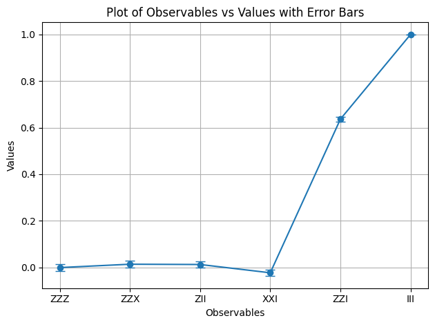
เราจะเห็นว่า observable $ZZI$ และ $III$ มีค่าความคาดหวังเท่ากับ 1 เนื่องจาก $ZZI$ ให้เครื่องหมายลบสองครั้งที่หักล้างกัน และ $III$ ทำหน้าที่เป็น identity ทำให้สถานะ GHZ ไม่เปลี่ยนแปลง ส่วน observable ที่เหลือมีค่าความคาดหวังเท่ากับ 0 เพราะตัวดำเนินการ $Z$ ของมันให้เครื่องหมายลบจำนวนคี่ หรือตัวดำเนินการ $X$ พลิก qubit จำนวนหนึ่งจนทำให้สถานะที่ซ้อนทับกันตั้งฉากกัน

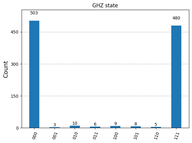
ต่อไปเราจะพล็อตผลลัพธ์ของ Sampler

counts_list = results_sampler[0].data.meas.get_counts()
print(counts_list)
print(f"Outcomes : {counts_list}")
display(plot_histogram(counts_list, title="GHZ state"))

{'111': 480, '000': 503, '101': 8, '100': 9, '001': 3, '011': 6, '010': 10, '110': 5}
Outcomes : {'111': 480, '000': 503, '101': 8, '100': 9, '001': 3, '011': 6, '010': 10, '110': 5}

2.5 ขยายไปสู่จำนวน Qubit ขนาดใหญ่

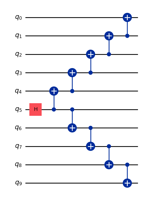
ในการคำนวณเชิงควอนตัม งานระดับ utility-scale มีความสำคัญมากต่อการพัฒนาสาขานี้ งานดังกล่าวต้องการการคำนวณในขนาดที่ใหญ่กว่ามาก โดยอาจใช้ Circuit ที่มี qubit มากกว่า 100 ตัวและ Gate มากกว่า 1,000 ตัว ตัวอย่างนี้เป็นก้าวเล็กๆ ในทิศทางนั้น โดยขยายปัญหา GHZ ไปที่ $n=10$ Qubit ใช้กระบวนการ Qiskit patterns และสิ้นสุดด้วยการวัดค่าความคาดหวัง $\langle Z_0 Z_i \rangle$

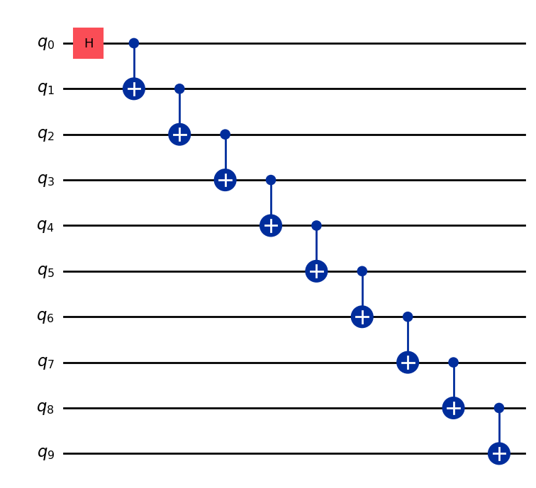
ขั้นตอนที่ 1 แมปปัญหา

เขียนฟังก์ชันที่คืนค่า QuantumCircuit ที่เตรียมสถานะ GHZ ขนาด $n$ Qubit (โดยพื้นฐานคือ Bell state ที่ขยายออก) จากนั้นใช้ฟังก์ชันนั้นเตรียมสถานะ GHZ ขนาด 10 Qubit และรวบรวม observable ที่จะวัด

def get_qc_for_n_qubit_GHZ_state(n: int) -> QuantumCircuit:

    qc = QuantumCircuit(n) 
    qc.h(0)
    for i in range(n-1):
        qc.cx(i, i+1)
    return qc
n = 10
qc_n_GHZ = get_qc_for_n_qubit_GHZ_state(n)
qc_n_GHZ.draw("mpl")

ต่อไปให้แมปไปยัง operator ที่สนใจ ตัวอย่างนี้ใช้ตัวดำเนินการ ZZ ระหว่าง Qubit เพื่อตรวจสอบพฤติกรรมเมื่อ Qubit อยู่ห่างกันมากขึ้น ค่าความคาดหวังที่ผิดพลาด (เสียหาย) มากขึ้นระหว่าง Qubit ที่อยู่ไกลกันจะบ่งบอกถึงระดับของ noise ที่มีอยู่

# ZZII...II, ZIZI...II, ... , ZIII...IZ
operator_strings = [
    "Z" + i * "I" + "Z" + "I" * (n-i-2) for i in range(n-1) 
]
print(operator_strings)
print(len(operator_strings))

operators = [SparsePauliOp(operator) for operator in operator_strings]

['ZZIIIIIIII', 'ZIZIIIIIII', 'ZIIZIIIIII', 'ZIIIZIIIII', 'ZIIIIZIIII', 'ZIIIIIZIII', 'ZIIIIIIZII', 'ZIIIIIIIZI', 'ZIIIIIIIIZ']
9

ขั้นตอนที่ 2 ปรับแต่งปัญหาให้พร้อมสำหรับการรันบน quantum Backend

แปลง Circuit และ observable ให้ตรงกับ ISA ของ Backend

# Convert to an ISA circuit and layout-mapped observables.
pm = generate_preset_pass_manager(backend=backend, optimization_level=2)
isa_circuit = pm.run(qc_n_GHZ) 
isa_operators_list = [operator.apply_layout(isa_circuit.layout) for operator in operators]

ขั้นตอนที่ 3 รันบน Backend

ส่ง job และถ้ารันบน hardware จริงให้เปิดใช้งานการระงับข้อผิดพลาดด้วยเทคนิคที่เรียกว่า dynamical decoupling. ค่า resilience level กำหนดระดับความยืดหยุ่นในการรับมือกับข้อผิดพลาด ค่าที่สูงขึ้นจะให้ผลลัพธ์ที่แม่นยำกว่า แต่ใช้เวลาประมวลผลนานกว่า ดูคำอธิบายเพิ่มเติมเกี่ยวกับตัวเลือกที่ตั้งไว้ในโค้ดต่อไปนี้ได้ที่ Configure error mitigation for Qiskit Runtime.

# Submit the circuit to Estimator
job = estimator.run([(isa_circuit, isa_operators_list)])
job_id = job.job_id()

/Users/jma/miniconda3/envs/3122/lib/python3.12/site-packages/qiskit_ibm_runtime/fake_provider/local_service.py:187: UserWarning: The resilience_level option has no effect in local testing mode.
  warnings.warn("The resilience_level option has no effect in local testing mode.")

ขั้นตอนที่ 4 ประมวลผลผลลัพธ์

เพื่อให้เข้าใจพฤติกรรมของสถานะควอนตัมที่พันกัน (entangled) บน hardware จริงได้ดีขึ้น เราจะวิเคราะห์ความสัมพันธ์เป็นคู่ (pairwise correlation) ระหว่าง Qubit ในฐาน Z โดยเฉพาะเราจะดูค่าความคาดหวัง ⟨Z₀Zᵢ⟩ ซึ่งวัดความแข็งแกร่งของความสัมพันธ์ระหว่าง Qubit 0 กับ Qubit i แต่ละตัว โดยเราจะพล็อต:

$$\langle Z_i Z_0 \rangle / \langle Z_1 Z_0 \rangle$$

คาดว่าจะเห็นค่าอะไรในกราฟสำหรับ $\langle Z_i Z_0 \rangle / \langle Z_1 Z_0 \rangle$?

ตัวเลือก:

a) ลดลงเมื่อ $i$ เพิ่มขึ้น

b) คงที่ที่ 1

c) มีความเบี่ยงเบนเล็กน้อยรอบๆ 1

d) สลับกันระหว่าง 1 และ 0 สำหรับค่า $i$ คี่และคู่

data = list(range(1, len(operators) + 1))  # Distance between the Z operators
result = job.result()[0]
values = result.data.evs  # Expectation value at each Z operator.
values = [
    v / values[0] for v in values
]  # Normalize the expectation values to evaluate how they decay with distance.

plt.plot(data, values, marker="o", label=f"{n}-qubit GHZ state")
plt.xlabel("Distance between qubits $i$")
plt.ylabel(r"$\langle Z_i Z_0 \rangle / \langle Z_1 Z_0 \rangle $")
plt.legend()
plt.show()

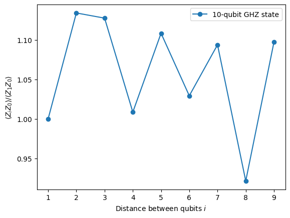
จากกราฟนี้เราสังเกตว่า $\langle Z_0 Z_i \rangle$ แกว่งรอบค่า 1 แม้ว่าในการจำลองแบบสมบูรณ์แบบ ค่า $\langle Z_0 Z_i \rangle$ ทั้งหมดควรเป็น 1

อย่างที่เห็น ผลลัพธ์ของการทดลอง 10 Qubit ค่อนข้างดี แต่ยังคงมีข้อผิดพลาดอยู่บ้าง วิธีหนึ่งในการปรับปรุงผลลัพธ์คือการสร้างสถานะ GHZ ให้มีประสิทธิภาพมากขึ้น

โดยปกติเราจะสร้างสถานะ GHZ ด้วยลำดับ CNOT gate แบบขั้นบันได แต่เราสามารถสร้างสถานะ GHZ ได้อย่างมีประสิทธิภาพมากกว่า โดยลด 2-qubit depth จาก n เหลือ n/2 หรือน้อยกว่า

metric สำคัญอย่างหนึ่งที่ใช้ benchmark ว่าผลลัพธ์จะแม่นยำแค่ไหนหรือมี noise น้อยแค่ไหนสำหรับ Circuit คือ 2-qubit gate depth เพราะอัตราข้อผิดพลาดของ 2-qubit gate (~10 เท่าของ single qubit gate) เป็นตัวครอบงำข้อผิดพลาดทั้งหมดของ Circuit ใช้โค้ดต่อไปนี้เพื่อดู 2-qubit gate depth ของ Circuit

qc.depth(lambda x: x.operation.num_qubits == 2)

def better_ghz(n):
    "fan out"
    s = int(n / 2)
    qc = QuantumCircuit(n)
    qc.h(s)
    for m in range(s, 0, -1):
        qc.cx(m, m - 1)
        if not (n % 2 == 0 and m == s): 
            qc.cx(n - m - 1, n - m)
    return qc

better_ghz(n).draw("mpl")

# Check 2-qubit gate depth before transpilation
qc_better_ghz = better_ghz(n)
qc_better_ghz.depth(lambda x: x.operation.num_qubits == 2)

5

สิ่งที่น่าสนใจคือเราสามารถลด quantum depth ของ Circuit ที่ต้องการรันได้เพียงแค่คิดหาวิธีโปรแกรมที่แตกต่างออกไป อย่างไรก็ตาม จะมีสถานการณ์และ algorithm ที่เราพึ่งพากลเม็ดเหล่านี้ไม่ได้ นั่นคือจุดที่ Transpiler เข้ามามีประโยชน์ มันช่วยให้เราปรับแต่งทุกด้านเหล่านี้ได้อย่างมีประสิทธิภาพ เพื่อที่เราจะได้ไม่ต้องกังวลกับมันมากเกินไป

3. การเข้ารหัสข้อมูล

3.1 Amplitude encoding

หลังจากที่เราเห็นวิธีสร้าง quantum Circuit แล้ว มาสำรวจกันว่าเราจะเข้ารหัสข้อมูลแบบคลาสสิกลงในสถานะควอนตัมได้อย่างไร วิธีหนึ่งที่ทรงพลังคือ amplitude encoding ที่ amplitude ของสถานะควอนตัมแทนค่าองค์ประกอบของเวกเตอร์แบบคลาสสิก

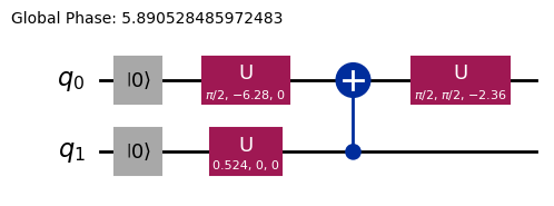
ลองพิจารณาตัวอย่างง่ายๆ สมมติว่าเราต้องการเข้ารหัสเวกเตอร์แบบคลาสสิก

$$\vec{x} = \begin{bmatrix} x_0 \\ x_1 \\ x_2 \\ x_3 \end{bmatrix}$$

ลงใน quantum state ของ Qubit สองตัว เป้าหมายคือเตรียม quantum state:

$$\ket{\psi} = x_0\ket{00} + x_1\ket{01} + x_2\ket{10} + x_3\ket{11}$$

โดยที่ $x_0, x_1, x_2, x_3 \in \mathbb{R}$ (หรือ $\mathbb{C}$) และเวกเตอร์ถูก normalize ให้:

$$|x_0|^2 + |x_1|^2 + |x_2|^2 + |x_3|^2 = 1$$

ทีนี้ลองพิจารณาตัวอย่างเฉพาะ: $\vec{x} = [0.8924, 0.3696, 0.2391, 0.0990]$

จากนั้น quantum state ที่สอดคล้องกันคือ:

$$\begin{aligned} \ket{\psi} &= 0.8924\,\ket{00} + 0.3696\,\ket{01} + 0.2391\,\ket{10} + 0.0990\,\ket{11} \end{aligned}$$

สถานะนี้สามารถเตรียมได้โดยใช้ rotation gate $R_y$ ที่มุม $\pi/6$ และ $\pi/4$ สำหรับ Qubit 0 และ 1 ตามลำดับ

from qiskit import QuantumCircuit
from qiskit_aer import AerSimulator
import numpy as np

qc = QuantumCircuit(2)

qc.ry(np.pi / 6, 0)
qc.ry(np.pi / 4, 1)

simulator = AerSimulator()
qc.save_statevector()
result = simulator.run(qc).result()
statevector = result.get_statevector()

print("Statevector:", statevector)
qc.draw(output="mpl")

Statevector: Statevector([0.8923991 +0.j, 0.23911762+0.j, 0.36964381+0.j,
             0.09904576+0.j],
            dims=(2, 2))

from qiskit.quantum_info import Statevector

# Define our vector
v = np.array([0.8924,  0.3696, 0.2391, 0.0990]) 
v = v/np.linalg.norm(v)
# Create a statevector from the vector
state = Statevector(v)

# Initialize a quantum circuit with 2 qubits
qc = QuantumCircuit(2)
qc.initialize(state.data, [0, 1])

# Optional: simulate the state
print("Statevector:", state)

# Visualize the circuit
qc.decompose().decompose().decompose().decompose().decompose().draw("mpl")

Statevector: Statevector([0.89242154+0.j, 0.36960892+0.j, 0.23910577+0.j,
             0.09900239+0.j],
            dims=(2, 2))

เราได้เห็นวิธีเข้ารหัสข้อมูลโดยใช้ rotation gate แล้ว

3.2 Angle encoding และ parametrized circuits

วิธีหนึ่งที่น่าสนใจในการเข้ารหัสข้อมูลลงในคอมพิวเตอร์ควอนตัมคือการออกแบบ quantum Circuit ที่ประกอบด้วยมุมการหมุน $\vec{\theta}$ หรือพารามิเตอร์ที่ปรับได้เพื่อแทน family ของฟังก์ชัน $f(\vec{\theta})$ ลองพิจารณา parametrized quantum circuit ต่อไปนี้:

from qiskit import QuantumCircuit
from qiskit.circuit import Parameter

# Define a symbolic parameter
theta = Parameter("θ")

qc = QuantumCircuit(2)
# We applied a parametrized RX gate
qc.rx(theta, 0)
qc.cx(0, 1)
qc.draw("mpl")

ทางคณิตศาสตร์เราสามารถวิเคราะห์ได้ว่า family ของฟังก์ชันที่เราแทนได้ด้วย Circuit นี้คืออะไร:

$$\text{CNOT}_{01} \, R_x^{\{0\}}(\theta) |00\rangle = \text{CNOT}_{01} \left( \cos(\theta/2)\ket{00} - i\sin(\theta/2)\ket{10} \right) = \cos(\theta/2)\ket{00} - i\sin(\theta/2)\ket{11}$$

จะเห็นชัดเจนว่าจำนวนสถานะที่เราแทนได้ด้วย quantum circuit นี้มีจำกัด เช่น เราไม่สามารถแทนสถานะ $\ket{10}$ หรือ $\ket{01}$ ได้ อย่างไรก็ตาม family ของสถานะที่เราแทนได้จะเริ่มขยายขึ้นเมื่อเราเพิ่ม rotation ในตำแหน่งที่เหมาะสม:

from qiskit import QuantumCircuit
from qiskit.circuit import Parameter

# Define a symbolic parameter
theta1 = Parameter("θ1")
theta2 = Parameter("θ2")

qc = QuantumCircuit(2)
qc.rx(theta1, 0)
qc.rx(theta2, 1)
qc.cx(0, 1)
qc.draw("mpl")

ในกรณีนี้ quantum state ที่เราจะแทนได้คือ:

\begin{align*} \text{CNOT}_{01} \, R_x^{\{1}}(\theta_2) R_x^{\{0}}(\theta_1) \ket{00} &= \text{CNOT}_{01} \, R_x^{\{1}}(\theta_2)\left( \cos(\theta_1/2)\ket{00} - i\sin(\theta_1/2)\ket{10} \right) \\ &= \text{CNOT}_{01}\left( \cos(\theta_1/2)\cos(\theta_2/2)\ket{00} - i\cos(\theta_1/2)\sin(\theta_2/2)\ket{01} \right. \\ &\quad \left. - i\sin(\theta_1/2)\cos(\theta_2/2)\ket{10} + \sin(\theta_1/2)\sin(\theta_2/2)\ket{11} \right) \\ &= \cos(\theta_1/2)\cos(\theta_2/2)\ket{00} - i\cos(\theta_1/2)\sin(\theta_2/2)\ket{01} \\ &\quad + \sin(\theta_1/2)\sin(\theta_2/2)\ket{10} - i\sin(\theta_1/2)\cos(\theta_2/2)\ket{11} \end{align*}

เราจะเห็นว่า Circuit นี้สร้าง family ของ quantum state ที่กว้างกว่า Circuit ก่อนหน้า โดยเฉพาะตอนนี้มันสามารถสร้างสถานะที่มี amplitude ไม่เป็นศูนย์สำหรับ $\ket{01}$ หรือ $\ket{10}$ ซึ่งทำไม่ได้กับ Circuit ข้างต้น อย่างไรก็ตาม Circuit นี้ยังไม่ใช่ตัวสร้าง quantum state แบบ universal แม้ว่ามันอาจมี expressiveness เพียงพอสำหรับการออกแบบ Circuit ที่มีความยืดหยุ่นพอในการแทนฟังก์ชันบางอย่าง โดยทั่วไปยิ่งเราเพิ่มพารามิเตอร์อิสระ (มุม) มากขึ้น Circuit ก็จะมี expressiveness มากขึ้นในการประมาณ quantum state ที่กำหนดใดๆ

Ansatzes และ Circuit library

วงจรควอนตัมแบบมีพารามิเตอร์ชนิดนี้สามารถนำไปสร้าง Ansatzes ซึ่งเป็นสถานะควอนตัมทดลองที่ใช้ประมาณค่าคำตอบของปัญหาต่าง ๆ Ansatzes เหล่านี้เป็นส่วนประกอบหลักของ Variational Quantum Algorithms ซึ่งเป็นกลุ่มของอัลกอริทึมไฮบริดควอนตัม-คลาสสิกที่ใช้คอมพิวเตอร์ควอนตัมในการประเมินฟังก์ชันต้นทุน และใช้ตัวปรับค่าแบบคลาสสิกในการลดค่าดังกล่าว เราจะลงรายละเอียดเรื่องนี้ในหน่วยถัดไป แต่ตอนนี้ขอแนะนำวิธีสร้าง ansatz อย่างง่ายโดยใช้ Circuit library ใน Qiskit ก่อน

from qiskit.circuit.library import efficient_su2

SU2_ansatz = efficient_su2(4, su2_gates=["rx", "y"], entanglement="linear", reps=1)
SU2_ansatz.decompose().draw(output="mpl")

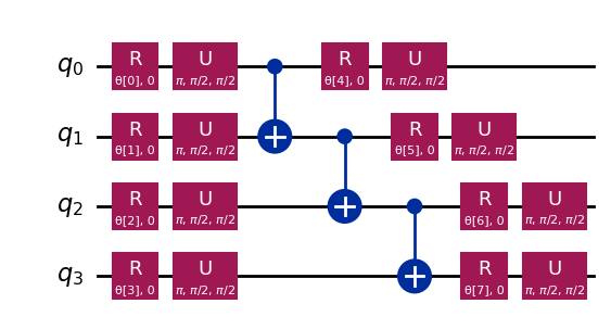
เราได้เห็นวิธีสร้าง Ansatz อย่างง่ายโดยใช้ฟังก์ชัน efficient_su2 จาก qiskit.circuit.library ซึ่งสามารถสร้างสถานะควอนตัมได้หลากหลายรูปแบบด้วยการปรับพารามิเตอร์ $\vec{\theta}$

บทสรุป

ในโน้ตบุ๊กนี้ เราได้เรียนรู้วิธีสร้าง Circuit ควอนตัม ตั้งแต่การสร้าง Gate ควอนตัม ไปจนถึงการกำหนดและวัด observable และวิธีรัน Circuit เหล่านี้อย่างมีประสิทธิภาพทั้งบน simulator และฮาร์ดแวร์ควอนตัมจริง นอกจากนี้เราก็ได้เห็นความสำคัญของการออกแบบ Circuit อย่างรอบคอบเพื่อลดข้อผิดพลาดเมื่อทำงานกับอุปกรณ์ควอนตัมจริง รวมถึงกลยุทธ์ในการขยาย Circuit ไปยัง Qubit จำนวนมากขึ้น โดยเฉพาะผ่านตัวอย่าง GHZ state นอกจากนี้เรายังได้สำรวจเทคนิคต่าง ๆ ในการเข้ารหัสข้อมูลคลาสสิกลงในสถานะควอนตัม ทั้ง amplitude encoding และ angle encoding ด้วยความรู้เหล่านี้ทั้งหมด ตอนนี้เราพร้อมที่จะก้าวไปยัง session ถัดไปและเริ่มทำงานกับอัลกอริทึมควอนตัมได้เลย

การติดตั้ง Qiskit Code Assistant ใน VSCode

คลิก ลิงก์ แล้วทำตามขั้นตอนที่ระบุไว้

โบนัส: Quantum Teleportation

เมื่อได้ยินคำว่า quantum teleportation หลายคนอาจนึกถึงเทคโนโลยีไซไฟในอนาคตที่สามารถย่อยวัตถุในจุดหนึ่งแล้วส่งไปปรากฏในอีกที่หนึ่ง แต่ความจริงแล้ว quantum teleportation ไม่ได้เป็นแบบนั้น สิ่งที่ถูก teleport ไม่ใช่สสาร แต่เป็นข้อมูล

Quantum teleportation คือโปรโตคอลที่ช่วยให้สามารถถ่ายโอนสถานะควอนตัมของ Qubit จากตำแหน่งหนึ่งไปยังอีกตำแหน่งหนึ่ง แม้การถ่ายโอนนี้ดูเหมือนเกิดขึ้นทันที แต่ก็ไม่ได้ละเมิดกฎฟิสิกส์ แล้วเป็นไปได้อย่างไร? มาลองทำความเข้าใจกัน

Quantum teleportation คือโปรโตคอลที่ช่วยให้ผู้ส่ง (Alice) สามารถส่งสถานะ $|\psi\rangle$ ของ Qubit q ไปยังผู้รับ (Bob) โดยใช้ทรัพยากรสำคัญสองอย่าง ได้แก่ คู่ Qubit ที่พันกัน (entangled pair) a และ b ที่ใช้ร่วมกัน และบิตคลาสสิกสองบิต c0 กับ c1 สำหรับการสื่อสาร

โดยหลักแล้วโปรโตคอลต้องการ:

• q: Qubit ของ Alice ซึ่งเริ่มต้นอยู่ในสถานะ $|\psi\rangle$ ที่ต้องการ teleport
• a: ครึ่งหนึ่งของคู่ Qubit ที่พันกันของ Alice
• b: ครึ่งหนึ่งของคู่ Qubit ที่พันกันของ Bob
• c0, c1: บิตคลาสสิกสำหรับเก็บผลการวัดของ Alice

แล้วมันทำงานอย่างไร? ขั้นตอนมีดังนี้

1. เตรียมสถานะ $|\psi\rangle$ ของ Alice บน q: เราจะสร้างสถานะเฉพาะอย่าง $|+\rangle$ เพื่อใช้ในการตรวจสอบ
2. สร้าง entanglement: สร้าง Bell pair ระหว่าง a และ b
3. การดำเนินการของ Alice: Alice ทำ "Bell measurement" บน Qubit สองตัวของเธอ (q และ a) และเก็บผลลัพธ์คลาสสิกไว้ใน c0 และ c1
4. การสื่อสารแบบคลาสสิก: Alice ส่งบิตคลาสสิกสองบิต (c0, c1) ไปให้ Bob
5. การแก้ไขของ Bob: Bob ใช้ Gate ควอนตัม (X และ/หรือ Z) กับ Qubit ของเขา (b) โดยขึ้นอยู่กับค่า c0 และ c1 ที่ได้รับ

ถ้าทำถูกต้องทุกขั้นตอน Qubit b ของ Bob จะอยู่ในสถานะ $|\psi\rangle$ ซึ่งเป็นสถานะดั้งเดิมของ q ของ Alice!

สำหรับคำอธิบายและการสำรวจ quantum teleportation เชิงลึกมากขึ้น รวมถึงการอธิบายทางคณิตศาสตร์ว่าทำไมโปรโตคอลนี้ถึงใช้งานได้ สามารถดูได้จากแหล่งเรียนรู้ IBM Quantum: Quantum Teleportation ซึ่งเป็นส่วนหนึ่งของคอร์ส Basics of Quantum Information

import matplotlib.pyplot as plt
from qiskit import QuantumCircuit, QuantumRegister, ClassicalRegister
from qiskit_aer import AerSimulator
from qiskit.visualization import plot_histogram, plot_bloch_multivector

# Define individual quantum registers for each qubit
q = QuantumRegister(1, name='q')  # message qubit
a = QuantumRegister(1, name='a')  # Alice's entangled qubit
b = QuantumRegister(1, name='b')  # Bob's entangled qubit

# Classical register for Alice's measurements
cr_alice = ClassicalRegister(2, name='c_alice')

# Create quantum circuit
teleport_qc = QuantumCircuit(q, a, b, cr_alice, name='Teleportation')

# Step 1: Prepare message state |+⟩ on q
teleport_qc.h(q[0])
teleport_qc.barrier()

# Step 2: Create entanglement between a and b
teleport_qc.h(a[0])
teleport_qc.cx(a[0], b[0])
teleport_qc.barrier()

# Step 3: Alice's Bell measurement
teleport_qc.cx(q[0], a[0])
teleport_qc.h(q[0])
teleport_qc.barrier()

# Step 4: Alice measures q and a
teleport_qc.measure(q[0], cr_alice[0])
teleport_qc.measure(a[0], cr_alice[1])
teleport_qc.barrier()

# Step 5: Bob's conditional measurements
with teleport_qc.if_test((cr_alice[1], 1)):
    teleport_qc.x(b[0])
with teleport_qc.if_test((cr_alice[0], 1)):
    teleport_qc.z(b[0])

# Draw the circuit
teleport_qc.draw(output='mpl')

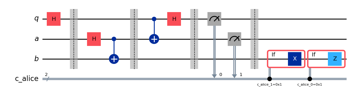
หลังจากรันโปรโตคอลแล้ว คำถามสำคัญคือ เราจะยืนยันได้อย่างไรว่า teleportation สำเร็จ? เราไม่สามารถ "มองเห็น" สถานะของ Qubit ของ Bob ได้โดยตรงหลังจากรันโปรโตคอล อย่างไรก็ตาม เนื่องจากเราเตรียมสถานะเริ่มต้นของ Alice ไว้ (เราเลือก $|+\rangle$) เราสามารถใช้การจำลองแบบพิเศษเพื่อตรวจสอบว่า Qubit b ของ Bob อยู่ในสถานะเดียวกันหรือไม่

เราจะใช้ AerSimulator พร้อม save_statevector เพื่อตรวจสอบว่า Qubit b ของ Bob ลงเอยด้วยสถานะเริ่มต้นของ Alice ($|+\rangle$) หรือเปล่า โดย simulator นี้จะคำนวณ state vector ควอนตัมขั้นสุดท้าย จากนั้นแสดงผลด้วย plot_bloch_multivector เพื่อให้เห็นภาพ Qubit ของ Bob (b) เทียบกับสถานะเริ่มต้นของ Alice (q)

# Simulate the teleportation circuit
sv_simulator = AerSimulator(method='statevector')
teleport_qc_sv = teleport_qc.copy()
teleport_qc_sv.save_statevector()

# Execute the circuit on the statevector simulator
job_sv = sv_simulator.run(teleport_qc_sv)
result_sv = job_sv.result()

# Get the final statevector
final_statevector = result_sv.get_statevector()
print("Visualizing final qubit states:")
display(plot_bloch_multivector(final_statevector))
print("Note that Alice's qubits have collapsed to |00⟩, |01⟩, |10⟩, or |11⟩, while Bob's qubit is in the original state |+⟩.")

Visualizing final qubit states:

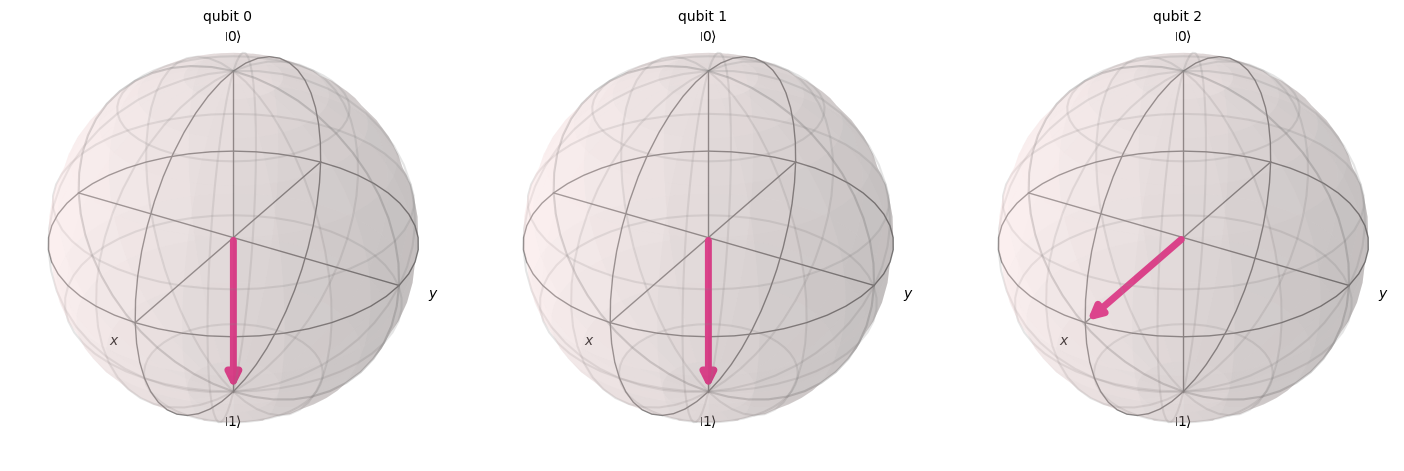
Note that Alice's qubits have collapsed to |00⟩, |01⟩, |10⟩, or |11⟩, while Bob's qubit is in the original state |+⟩.

จากภาพที่เห็น Qubit สองตัวแรก (ของ Alice) ได้ collapse ไปเป็น 0 หรือ 1 แล้ว ในขณะที่ Qubit ที่สาม (ของ Bob) ซึ่งแสดงในทรงกลม Bloch ที่สาม ชี้ไปตามแกน x ซึ่งบ่งบอกว่าอยู่ในสถานะ $|+\rangle$ แสดงว่าเราได้ implement โปรโตคอล quantum teleportation สำเร็จแล้ว!

สรุป

ณ จุดนี้ขอสรุปสิ่งที่เราทำได้สำเร็จอย่างรวดเร็ว:

• Alice ได้ส่ง สถานะควอนตัมที่ไม่รู้จัก ไปยัง Bob
• ไม่มีอนุภาคทางกายภาพใดถูกถ่ายโอน
• สถานะเดิมบน Qubit ของ Alice ถูกทำลาย ซึ่งสอดคล้องกับทฤษฎีบท No-Cloning

อย่างไรก็ตาม quantum teleportation ยังคงต้องใช้การสื่อสารแบบคลาสสิก (ผลการวัดของ Alice ที่ส่งไปยัง Bob) ซึ่งอธิบายได้ว่าทำไมกระบวนการนี้จึงไม่อนุญาตให้มีการส่งข้อมูลที่เร็วกว่าแสง และสอดคล้องอย่างสมบูรณ์กับกฎทางฟิสิกส์ที่รู้จักทั้งหมด